4 Applications

⊕ Go to: Table of contents Chapters: 1 2 3 4 5

4-1 The first Poisson application to goals
4-2 The 2018/2019 season of five leagues

The analysis of goals in Moroney (1951) is known as the first statistical analysis of goals in football matches. Moroney, M., J., 1951, Facts from figures. 3rd edition, 1973 reprint,London:Penguin. This chapter describes his application of the Poisson model to a set of matches.

It also allows you to evaluate how well the Poisson distribution describes the actual distribution of goals across matches for the 2018/2019 season in the highest professional football divisions of England, Spain, Germany, Italy and France. This part has interactive elements which work best on larger screens. They may not work on your mobile phone.

4-1 The first Poisson application to goals

It seems that the first application of the Poisson model to goals in matches appears in Moroney (1951). His book contains many examples of different statistical analyses in different fields.⊕ Back to top

Chapter 8 of his book includes applications of the Poisson model to data. One of them concerns the number of goals by teams in football matches. Moroney explains why the Poisson model may be appropriate to model the number of goals per match as follows: Page 96 of Moroney (1951)

"The number of goals scored in a football match is another case of isolated events in a continuum of time. We know how many times a goal was scored in a match but we do not know how many times a goals wasn't scored during the match."

He further explains that the Poisson distribution provides an approximation of the goals per match instead of an exact description. Page 101 of Moroney (1951)

"Again, we should not expect the Poisson distribution to give a perfect description of the number of goals scored per team per match at football, since the expected number of goals depends, among other things, on which teams are opposed, on the weather conditions, and so on."

Using information of 480 matches during which teams scored a total of 812 goals he calculated the frequencies of a random variable with a Poisson distribution and a mean of 1.7 goals per team per match. 812 goals in 480 matches gives and a sample mean of 1.7 goals per match. No source appears available for the information about these matches. Unless proven otherwise, it seems safe to assume that it concerns matches of the 1950/1951 season of the Scottish A League for two reasons. The profile of a candidate that is well-positioned to verify and, possibly, disprove this claim is a curious person with an interest in history and football living in England's Leicester area. First, note that 16 teams means 480 matches in a double-round robin tournament. Second, the mean and standard deviation of the number of goals per match in his book are remarkably close to those from matches by the 16 teams in the 1950/1951 season of the Scottish A League.

Figure 4-1 shows the results of his analysis—a comparison between the actual number of matches with the modelled number of matches for a given number of goals in match.

Figure 4-1: Number of matches by goals per team — Poisson distribution. Figure 4-1 corresponds to panel (a) in Figure 36 on page 103 of Moroney's book. The dark and light bars correspond to the reported "Observed Frequencies" and "Poisson Frequencies" at the bottom of page 101, respectively.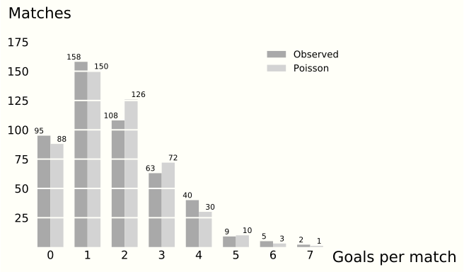

We return to Moroney's analysis in section 5-1.

4-2 The 2018/2019 season of five leagues

The simple Poisson model only requires the average number of goals per match for calculating of probabilities. In some cases this provides a reasonable description of the distribution of matches during a season by the number of scored goals. This is not always the case though.⊕ Back to top

In this section you can check yourself how a simple Poisson model describes the distribution of goals in matches for the 2018/2019 seasons in England, Spain, Italy, Germany and France.The information about matches for these five seasons is available in files for download at football-data.co.uk. At the time of writing this section the numbers of goals and counter-goals by team in these files equal those in the end-of-season-tables available at the football statistics site of rsssf.com.

Click a box in the table at the end of this section to see how the Poisson distribution describes the distribution of goals across matches for the season you are interested in. After clicking a box, histograms like that in Figure 4-1 appear together with some descriptive statistics.

We distinguish between goals scored by the home team and goals scored by the visiting team, respectively. This means that we assume statistical independence between goals that home teams score and goals that visiting teams score.

The descriptive statistics are the goals per match (the sample mean), variance, dispersion, minimum, maximum and correlation, respectively. The goals per match is the only information used for calculating the probabilities of the Poisson model.

The variance is a measure of variation in the number of goals across matches. One assumption of the Poisson distribution is that the expectation of a variable with a Poisson distribution is equal to its variance. The ratio of the variance and the mean being close to one or not informs us about the plausibility of this assumption. We denote this ratio by dispersion.Note that dispersion is an estimate of the true (and unobserved) dispersion. As such, it is possible to observe some under-dispersion or over-dispersion in the data even if a Poisson distribution generated the data.

You can check yourself whether assuming Poisson equi-dispersion of goals across matches is plausible for a given set of goals in matches. By comparing different leagues you will see that the Poisson model histograms are visually closer to the histograms of the actual goals for dispersions closer to one.

The correlation measures the association between goals by the home team and goals by the visiting team. A positive value means that matches with more goals for the home team tend to show more goals for the visiting team. Similarly, a negative value means that matches with less goals scored by the home team tend to show more goals scored by the visiting team. We show two different measures of correlation. The Pearson correlation assumes the association between "home goals" and "visiting goals" is linear while the Spearman correlation uses the goal-based-rank-ordering of matches to measure association.

Like dispersion, the correlations we calculate are estimates and for this reason it is possible to observe some correlation in the data even if the true (and unobserved) Poisson distributions of goals by home teams and goals by visiting teams are independent.If the goals that home teams score are statistically independent from the goals that visiting teams score, then the theoretical correlation between them is zero.

If you select a country by clicking on one of the five boxes above, then two figures will appear. The left and right figures show the modeled share of matches by home-team-goals and by visiting-team-goals, respectively. Both figures also show the actually observed shares of matches.

Some patterns appear for all countries. First,visually, the simple Poisson model appears to reflect the number of goals across matches reasonably well.This is just a visual inspection and one can use, for example, a Chi-squared test to formally assess the differences between the modeled shares and the actual shares. Second, a larger share of matches with zero goals appears in the right figure. This reflects an away disadvantage or home advantage in matches: it is more difficult to score a goal in away matches for teams than in their own stadium. Third, the peaks of the distributions appear at one goal. The most frequent number of goals by either the home team or the visiting team is one. This peak is less pronounced for goals by visiting teams in France and Spain where similar shares appear for one and no goal.

The models of home goals for Germany and Spain show over-dispersion (1.27) and under-dispersion (0.9), respectively. The modeled share of matches with zero goals is higher (lower) than the actual share in case of under-dispersion (over-dispersion). Recall that the Poisson model assumes that dispersion is equal to one. For Germany, the Poisson model appears to under-estimate the observed share of matches without home goals. We observe the opposite for Spain which shows under-dispersion in the data on home goals.Note that dispersion is model-specific — it compares the dispersion in the data with the dispersion implied by the model.

England and Germany show the largest correlations between goals by the home team and goals by the visiting team. They are negative and close to -0.20. It indicates a small tendency of matches to show a lower number of goals by the visiting team if we observe a large number of goals by the home team (and vice versa).

Overall, the simple Poisson model appears a reasonable description of the distribution of goals across matches for Italy while less so for Germany. Chapter 5 shows applications of Poisson models which allow different matches to have different Poisson distributions.