3 Uncertain goals per match
Go to: Table of contents
Chapters 1
2
3
4
5
3-1 Experiment and probability
3-2 The Bernoulli distribution
3-3 Opportunities and goals
3-4 The Poisson distribution
3-5 Ball possession as an opportunity
For modelling purposes we can consider goals in football matches as outcomes of a statistical experiment. Random variables describe outcomes in statistical experiments. Probability distributions describe the uncertainty across the possible outcomes of such variables. In this chapter we explain why the Poisson distribution often provides a reasonable description of how uncertainty distributes across the possible number of goals in a match.
3-1 Experiment and probability
Something happens if
we carry out an experiment. Suppose we repeat an experiment under as-identical-as-possible circumstances. If we get the same result each time, no matter how many repetitions of the experiment, then we can predict with certainty the outcome of the experiment. If the repetitions give different outcomes then we say that the experiment is unpredictable. In this case, chance affects the outcomes of our experiment.
Back to top
As an example, the Bernoulli trial is a well-known chance experiment. It is an experiment with exactly two outcomes—often classified as "Failure" and "Success".The sample space of an experiment contains all possible outcomes that can happen if you carry out an experiment. The sample space of a Bernoulli trial contains two outcomes. Either we get "Failure" or we get "Success". We don't know which outcome we will get but we know that we will only get one of these two outcomes. We describe this uncertainty by a probability p—usually p denotes the probability of "Success".
The probability p is a number which is at least zero and at most one. It indicates the degree of uncertainty about a possible outcome or event. If p equals one then the event is certain to happen. If it is zero then it is certain that it will not happen. A probability between zero and one shows the degree of uncertainty about whether the event will happen or not. Values close to one (zero) indicate a high probability that the event will (not) happen.
If we subtract the probability p from one, then we get 1-p. This number is also a probability. If p is the probability of an event to happen, then 1-p is the probability that the event will not happen. In a Bernoulli trial, 1-p is the probability of no "Success". It is the probability of "Failure".
3-2 The Bernoulli distribution
Something which does not change is constant. If something is not constant then it can take different values — it varies. Variables are useful to describe experiments. A variable can take different values. If the values a variable can take are not predictable then we say that the variable is a random variable. The field of statistics is concerned with random variables.
Back to top
Random variables have a probability distribution which relates its possible values to probabilities. It distributes uncertainty across the possible values which the random variable can take.The sample space of a random variable determines the number of possible values. Tossing a coin and throwing a dice are examples that help understanding how random variables describe the uncertainty of outcomes in an experiment.
If we toss a coin then either "Heads" or "Tails" appears up at the coin's face. We can use a random variable to describe the toss of a coin as an experiment. The random variable can take two possible values: "Heads" or "Tails".These two events describe the sample space of the experiment. We assume that either of these events occur with probability one.
How should we distribute the uncertainty we have about the outcome of the coin toss? We assume that it is equally likely to observe "Heads" as it is to observe "Tails". Because we are certain that only one of these two outcomes is possible this implies that "Heads" appears with probability one in two. Similarly, "Tails" appears with probability one in two.
These probabilities reflect the uncertainty we have about the two possible outcomes of tossing a coin. We say that the random variable which can take the values "Heads" or "Tails" has a Bernoulli distribution with probability one half.
More general, a random variable with two outcomes of which one occurs with probability p has a Bernoulli distribution with parameter p. Usually, the parameter p is unknown and needs to be determined, guessed or estimated. In our case, we assumed that the coin is "fair" meaning that observing "Heads" is as likely as observing "Tails". This assumption means that p is equal to one half because either "Heads" or "Tails" appears up at the coin's face with probability one.
Figure 3-1 shows the probability distribution for our experiment.
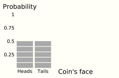
Figure 3-1: The Bernoulli distribution describing the uncertainty about the possible outcomes of tossing a coin (p =1/2).
We can use random variables to describe any statistical experiment. As another example, consider throwing a dice with six faces. This experiment has six possible outcomes: one dot, two dots, three dots, four dots, five dots or six dots show up, respectively. Assuming we are throwing a "fair" dice, each of these outcomes has a probability of one in six.
Figure 3-2 shows the probability distribution for this experiment. It describes the uncertainty of a dice throw by a one-in-six probability for each of the six possible numbers of dots.
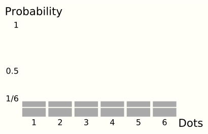
Figure 3-2: A discrete probability distribution (p=1/6) describing the uncertainty about the possible outcomes of throwing a dice.
The distributions in Figures 3-1 and 3-2 are distributions of uncertainty across discrete values. The numbers of goals in matches are values that are discrete—we don't see teams that score 1.2 or 0.7 goals in a match. The next section shows how to use the Bernoulli distribution for modelling the uncertainty about the number of goals in match.
3-3 Opportunities and goals
We can build on the Bernoulli distribution to describe uncertainty about the number of goals that teams score in matches. Suppose an opportunity arises during a match for a team and that this results in a goal with probability p=1/100.
We assume that the Bernoulli distribution describes the uncertainty about whether the opportunity results in a goal. Figure 3-3 shows this uncertainty.
Back to top
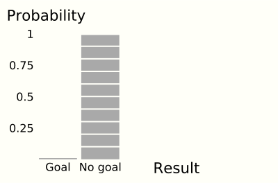
Figure 3-3: The Bernoulli distribution describing the uncertainty about whether an opportunity results in a goal or not (p=1/100).
Figure 3-3 shows a probability of 99/100 that the opportunity does not result in a goal. The probability of a goal is low and equal to 1/100 or one in hundred. Then, if hundred of such opportunities arise we may expect one goal. However, it is also possible to observe no goal at all or two goals, or any number of goals less than 101, no matter how unlikely this is.
The Binomial distribution describes the uncertainty about the results of repeating a given number of Bernoulli trials. We can use it to describe the uncertainty about the number of goals if, say, n=100 opportuntities arise during a match. This requires assuming that the probability of a goal is constant between opportunities and that the opportunities are independent.Two trials are dependent if knowledge of the outcome of one trial changes the probabilities of observing certain outcomes in the other trials. Trials are independent if they are not dependent.
Let's consider a football match with a fixed number of 100 opportunities of which each has a probability of one in hundred to result in a goal. We assume opportunities are independent from each other. That is, we assume the probabilities of "Goal" and "No goal" for future opportunities do not change if the current opportunity results in a goal or not. We further assume that we can describe the uncertainty about the number of goals in this match by a Binomial distribution with n=100 and p=1/100. Figure 3-4 shows this distribution. We don't show the probabilities for more than five goals as they are tiny.
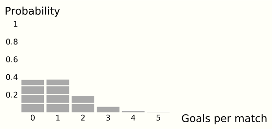
Figure 3-4: A Binomial distribution with n=100 and p=1/100
In this case, the probability that no goal results from the 100 opportunities is equal to 0.366. This means that the probability of observing at least one goal is 0.634—it is more likely than not to observe at least one goal. The probability that one goal results from the 100 opportunities is equal to 0.370. Similarly, the probability of two and three goals are equal to 0.18 and 0.06, respectively. The probability of 1, 2, or 3 goals is equal to 0.61, the sum of 0.37, 0.18 and 0.06. They make up the bulk of the 0.634 probability that at least one goals results from the opportunities.
The mass of the probability in Figure 3-4 appears around one goal. This is not a surprise because the expectation of this Binomial distribution is equal to the number of opportunities (n=100) times the probability (p=1/100) which is one goal. The expectation of a distribution is a measure of the "center" of the distribution, or the location of the distribution. In general, a Binomial distribition with n repetitions and probability p has expectation n*p.
3-4 The Poisson distribution
To apply the Binomial distribution to a real football match we need information about the number of opportunities and whether they result in a goal or not. However, we usually don't know how many opportunities arise in match. Also, in order to count the number of opportunities we would need a definition of opportunity.
Back to top
In this case, the Poisson distribution may give a reasonable approximation. The Poisson distribution is a popular distribution to model uncertainty about the number of occurences in an experiment, for example, goals by teams in football matches. It is relatively simple to apply and sometimes works reasonably well in describing uncertain outcomes—like goals in matches.The Poisson distribution owes its name to Siméon Denis Poisson who presented the derivation of this distribution in 1837. In 1711, Abraham DeMoivre provided a derivation of the probability that no event occurs for this distribution. The Poisson distribution gained importance in the analysis of data after Ladislaus von Bortkiewicz used it to investigate the number of Prussian soldiers who were kicked to death by horses and the number of child suicides, respectively. See Poisson, S. D., 1837, Recherches sur la Probabilité des Jugements en Matière Criminelle et en Matière Civile, Précédees des Regles Générales du Calcul des Probabilités, Paris: Bachelier; De Moivre, A., 1711, De Mensura Sortis, Philosophical Transactions of the Royal Society, vol.27, 213-264; Bortkiewicz, L., von, 1898, Das Gesetz der Kleine Zahlen, Leipzig: Teubner.
Poisson (1837) observed that in many cases the longer you wait for an event to happen the higher the probability that the event actually happens. To explore this, he assumed that the probability of an event is proportional to the length of the time interval. Then, the probability that an event happens is smaller for shorter time intervals.
Poisson investigated what happens if you start from a given time interval and repeatedly reduce the interval towards zero. For each reduced interval, Poisson calculated the occurences of 0, 1, 2, and so on, events. This way he found that a distribution which is now known as the Poisson distribution provides a reasonable approximation to the Binomial distribution.
To see why, note that it is always possible to repeat the reduction of time intervals often enough until the time intervals are so small that at most one event takes place. As an example, count the number of times that it rains during a given year. This is more than one if you do not live in an always-dry-place. Reduce the one-year-interval to twelve intervals of one month and count the number of times that it rains in each month. If one month has rainfall more than one once, reduce the number of months to weeks or days. You can continue this process until you find a length of interval in which it rains at most one time.
After splitting the year in intervals of a length for which it rains at most once in each interval we can describe the probability that it rains during an interval by a Bernoulli distribution (recall Figures 3-1 and 3-3). Now, let p be the probability of rainfall during an interval and we have split the year in n intervals. Then, we can describe the uncertainty about rainfall by a Binomial distribution with n intervals and a probability p of rainfall.
Poisson found that—what is now known as—the Poisson distribution provides a reasonable approximation of a Binomial distribution if n is large and p is small. This is a very useful result for analysing data because the Poisson distribution does not require n and p to be specified. The reason is that the Poisson distribution only needs the product n*p for determining the probabilities of a given amount of events occuring.These probabilities can be calculated with the probability mass function of the Poisson distribution: ... with ... the Poisson random variable, ... the number of events and ....
Suppose that you found that days are the time intervals during which rains at most once. Moreover, you think that the probability p of rainfall on a day is small, for example, because you are investigating rainfall in a dry region. Then, the Poisson distribution may give a reasonable approximation of the distribution of uncertainty about the number of possible days with rainfall during a year. In this case, you don't need to know the exact number n days and the exact probability p. To apply the Poisson distribution and describe uncertaity about rainfall, you only need a guess or estimate of the average number of days with rain for the period you are interested in (we used year as an example).
Hence, the Poisson distribution is attractive if you would like to apply the Binomial distribution but you don't know n and p but you have good reasons to think n is large and p is small.
In our case, using the Poisson distribution for modelling the number of goals in a match is an alternative to the Binomial distribution if the number of opportunities in a match is large and the probability that an opportunity results in a goal is small. This has great appeal because we usually don't know the number of opportunities in a match nor the number of times that opportunities result in a goal.
Hence, if we believe a match has many opportunities with small probabilities to result in a goal then the Poisson distribution is a good candidate for modeling the number of goals in a match. Opportunities in a match as a concept is a bit vague. There need to be many of them for the large-n-assumption of the Poisson distribution approximation to the Binomial distribution to hold. Maher (1982) suggested to think of ball possession as an opportunity and we show why this interpretation works in the next section.Maher, M. J., 1982, Modelling association football scores. Statistica Neerlandica, vol. 36, no.3, 109-118.
3-5 Ball possession as an opportunity
Until now we used opportunities to describe something that happens in matches which may or may not result in a goal. In this section we check whether we can think of ball possession as such an opportunity. Maher (1982) which we discuss further in Chapter 5 uses ball possession to motivate the Poisson approximation of a Binomial distribution.
Back to top
Suppose a team gains possession of the ball from its opponent in a match. This may or may not result in a goal with some probability. To simplify, we assume that only two things can happen: either the team scores a goal or not.
A book by Anderson and Sally (2013) reports an average of 190 ball possessions for teams in matches. They calculated this average using information of three Premier League seasons. See Anderson, C. and D. Sally, 2013, The Numbers Game. Why everything you know about football is wrong., 2nd edition, London:Penguin. They also note that an average of 0.74 in 100 possessions results in a goal. We can use these numbers to model the number of goals per match by a Binomial distribution and check whether the Poisson distribution reasonably approximates it.
First the Binomial distribution, let's assume we can describe the uncertainty about the number of goals in those matches by a Binomial distribution with n=190 and p=0.74/100. Now the Poisson distribution, let's consider n=190 large and p=0.74/100 small. We assume a Poisson distribution with an average of 1.406 goals per match (n*p=190*0.74/100=1.406).
Table 3-1 shows in percentages the probabilities of zero to six goals per match according to the Binomial distribution and its Poisson approximation.
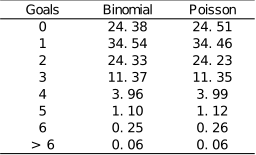
Table 3-1: Probabilities (%) of goals per match. The Binomial distribution with n=190 and p=74/10000 and its approximating Poisson distribution with n*p=1.406.
Table 3-1 shows, perhaps remarkably, small differences in the probabilities of a given number of goals per match between the Binomial distribution and its Poisson approximation. It supports Maher (1982) who suggested to think about ball possessions resulting in goals when applying the Poisson distribution to model the number of goals per match.